Interactive 1D Generative Models: From GANs to Diffusion

Introduction

This post is based on an exercise I developed for the Master in Computer Vision at the Computer Vision Center (CVC). The goal: understand GANs by working with 1D data instead of images.

Generative Adversarial Networks (GANs) are one of the most widely known algorithms in Machine Learning. Unlike discriminative models that learn $P(y \mid x)$, GANs are generative models that learn $P(x)$ directly—they learn to generate data.

While images are the most common application, training GANs on 1D data offers several advantages for learning:

1. Visualization: We can directly plot the real and generated distributions
2. Fast iteration: Training takes seconds, not hours
3. No GPU required: Everything runs in your browser
4. Clear convergence criteria: We know the exact target distribution

On Random Numbers

Let’s begin with a fundamental question: how are random numbers generated in your computer?

Perhaps surprisingly, computers don’t generate truly random numbers. They use pseudorandom number generators (PRNGs) that produce deterministic sequences that appear random. Given the same seed, a PRNG will always produce the same sequence:

>>> import numpy as np
>>> np.random.seed(42)
>>> np.random.rand()
0.3745401188473625
>>> np.random.rand()
0.9507143064099162

>>> np.random.seed(42)  # Reset seed
>>> np.random.rand()
0.3745401188473625     # Same value!

This determinism is actually useful for reproducibility—you can recreate exactly the same “random” experiment by setting the same seed.

The Inverse Transform Method

It’s relatively easy to generate uniformly distributed random numbers in $[0, 1]$ using algorithms like the Mersenne Twister. But what if we want samples from other distributions like Gaussian, Exponential, or something more complex?

One elegant solution is the inverse transform method. Given the cumulative distribution function (CDF) $F(x) = P(X \leq x)$, we can generate samples from the distribution by:

1. Sample $U \sim \text{Uniform}(0, 1)$
2. Return $X = F^{-1}(U)$

For example, the exponential distribution with rate $\lambda$ has CDF $F(x) = 1 - e^{-\lambda x}$, which gives us the inverse:

>>> import numpy as np
>>> lam = 0.5
>>> U = np.random.uniform(0, 1, 10000)
>>> X = -np.log(1 - U) / lam  # Exponential samples!

This is exactly what’s happening under the hood when you call np.random.exponential().

Higher Dimensions: The Manifold Hypothesis

Now here’s where it gets interesting. Consider images—say, $256 \times 256$ RGB images. Each image is a point in $\mathbb{R}^{256 \times 256 \times 3} = \mathbb{R}^{196608}$.

If we tried to uniformly sample this space:

>>> random_image = np.random.uniform(0, 255, (256, 256, 3))

We’d get noise. The number of possible images is $256^{196608}$—an astronomically large number. The vast majority of this space contains meaningless noise, not recognizable images.

Here’s the key insight: meaningful images lie on a lower-dimensional manifold. All images of dogs, for example, can be parameterized by a relatively small number of factors: breed, pose, lighting, background, etc. This is the Manifold Hypothesis.

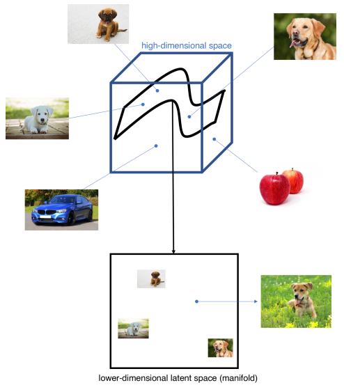
Different regions of the high-dimensional image space contain different categories of images. The manifold of dogs is distinct from the manifold of cats.

GANs as Learned Inverse CDFs

This brings us to the core idea: GANs learn the inverse CDF of complex distributions.

For simple distributions like Exponential, we can write $F^{-1}$ analytically. But for “the distribution of all dog images”? That’s intractable.

Instead, we let a neural network $G$ learn this transformation:

The Generator takes “easy” samples from a simple distribution (typically Gaussian) and transforms them into samples from the target distribution. It’s learning the inverse CDF implicitly!

A Game Theory Perspective

But how do we train $G$ without knowing $p_{\text{data}}$ explicitly? We only have samples from it.

The clever trick is to introduce a second network: the Discriminator $D$. These two networks compete in a minimax game:

• Discriminator $D$: Tries to distinguish real samples from fake ones. It wants $D(x) \to 1$ for real data and $D(G(z)) \to 0$ for fake data.
• Generator $G$: Tries to fool $D$. It wants $D(G(z)) \to 1$.

The Generator transforms noise into fake samples, while the Discriminator classifies real vs. fake.

Training Dynamics

The GAN training process can be visualized as follows:

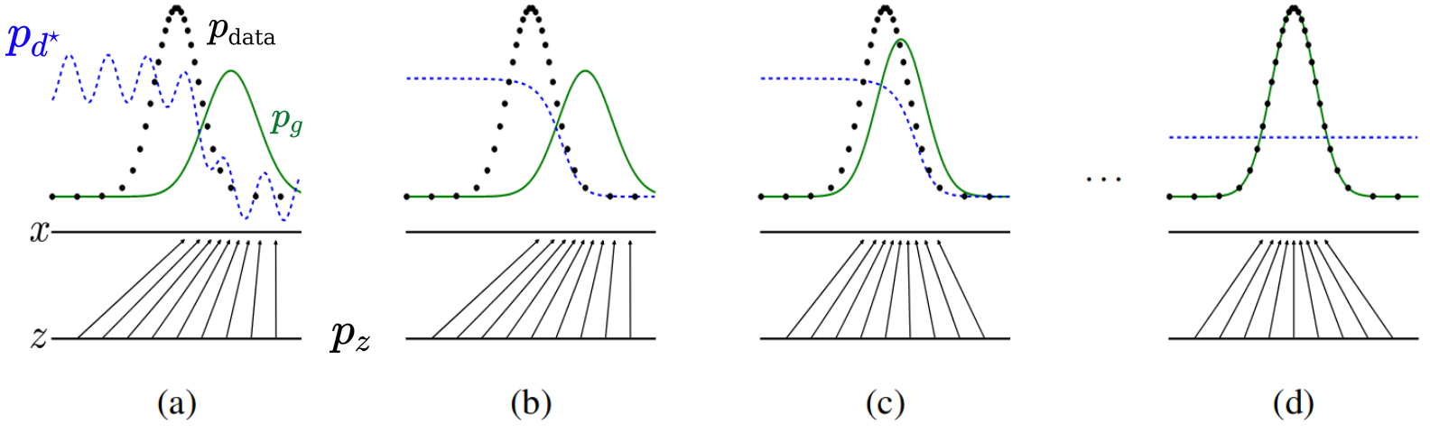
From the original GAN paper. As training progresses, the generated distribution (green) matches the real distribution (black dashed).

At Nash equilibrium, the Discriminator can no longer distinguish real from fake:

This means the optimal Discriminator outputs 0.5 for all inputs—it’s essentially guessing randomly.

Optimal Loss Values

When the GAN reaches equilibrium, we can derive the optimal loss values. Recall that we use Binary Cross-Entropy (BCE) loss:

For the Discriminator, we minimize the BCE for both real data (target $y=1$) and fake data (target $y=0$):

At equilibrium, $D^*(x) = 0.5$ for all inputs. Substituting:

For the Generator, using the non-saturating loss (explained below), we minimize:

At equilibrium:

The Training Algorithm

Here is the GAN training algorithm from the original paper:

The Non-Saturating Heuristic

There’s a practical issue with the original G loss. Early in training, when G produces garbage, D is very confident and outputs D(G(z)) ≈ 0. This means:

The gradient is nearly zero! G can’t learn because D is too good.

The solution is a clever heuristic: instead of minimizing $\log(1 - D(G(z)))$, we maximize $\log(D(G(z)))$:

# Original (saturating) - PROBLEMATIC
g_loss = -log(1 - D(G(z)))  # Gradient vanishes when D(G(z)) ≈ 0

# Non-saturating heuristic - USED IN PRACTICE
g_loss = -log(D(G(z)))      # Strong gradient even when D is confident

Both have the same optimum (G fools D), but the non-saturating version provides stronger gradients early in training.

Implementation in Python

Here’s how you’d implement this in PyTorch:

# Define loss criterion
criterion = nn.BCELoss()
real_label, fake_label = 1.0, 0.0

for epoch in range(num_epochs):
    for real_batch in dataloader:
        batch_size = real_batch.size(0)

        # === Train Discriminator ===
        D.zero_grad()

        # Real data
        label = torch.full((batch_size,), real_label)
        output = D(real_batch)
        loss_real = criterion(output, label)

        # Fake data
        noise = torch.randn(batch_size, latent_dim)
        fake = G(noise)
        label.fill_(fake_label)
        output = D(fake.detach())  # detach to avoid training G
        loss_fake = criterion(output, label)

        loss_D = loss_real + loss_fake
        loss_D.backward()
        optimizer_D.step()

        # === Train Generator ===
        G.zero_grad()

        label.fill_(real_label)  # G wants D to think fake is real
        output = D(fake)
        loss_G = criterion(output, label)  # Non-saturating!

        loss_G.backward()
        optimizer_G.step()

What to Observe in the Demo

When you run the training demo above, watch for:

1. Distribution Plot: The green histogram (Generated) should gradually match the blue histogram (Real)

2. Loss Plot:
   • G loss (green) should approach log(2) ≈ 0.693 (yellow dashed line)
   • D loss (blue) should approach 2·log(2) ≈ 1.386 (orange dashed line)
3. Discriminator Response:
   • D(x) for real data (blue) should start near 1 and drop to 0.5
   • D(G(z)) for fake data (green) should start near 0 and rise to 0.5
   • Both converging to 0.5 (yellow dashed line) means D can’t tell real from fake
4. Statistics Tracking:
   • Mean of generated samples (green) should approach the target mean (dashed)
   • Std of generated samples (orange) should approach the target std (dashed)

Common Failure Modes

Mode Collapse

Mode collapse occurs when G generates only a few samples (or even just one), regardless of the input noise. This happens because G finds a “safe” output that fools D, and D can’t provide useful gradients to encourage diversity.

In the demo, try making D much stronger than G (more layers, more neurons). You might see the generated distribution “collapse” to a narrow peak.

Convergence Failure

If the learning rate is too high, or the architectures are poorly matched, training may fail entirely:

• G produces garbage that D easily identifies
• Gradients vanish or explode
• Losses diverge rather than stabilize

Experiments to Try

Here are some experiments to deepen your understanding:

1. Bimodal Distribution: Can G learn both modes? Watch for mode collapse where G only captures one peak.

2. Increase G Depth: Does adding more layers help for complex distributions like the 3-Mixture?

3. Imbalanced Architectures: What happens if D is much stronger than G? Or vice versa?

4. Small Datasets: How few samples can the GAN learn from? Try 512 samples with a complex distribution.

5. Latent Dimension: Higher latent dimension gives G more capacity to express diverse outputs. But is more always better?

Interpolation in High Dimensions

Once trained, we can explore the latent space. But be careful with linear interpolation! In high dimensions, linear interpolation between two points passes through regions of low probability density.

The issue is the curse of dimensionality: in high-dimensional Gaussian space, most of the probability mass lies in a thin shell at a specific radius from the origin. Linear interpolation cuts through the low-density center.

Instead, use spherical linear interpolation (slerp):

where $\theta = \arccos\left(\frac{z_1 \cdot z_2}{|z_1||z_2|}\right)$

This keeps the interpolated points on the high-probability shell throughout the interpolation.

Real-World Example: Text-to-Image Models

This isn’t just theoretical—it matters for modern text-to-image models too! Here’s a comparison using SDXL Turbo, interpolating between two prompts:

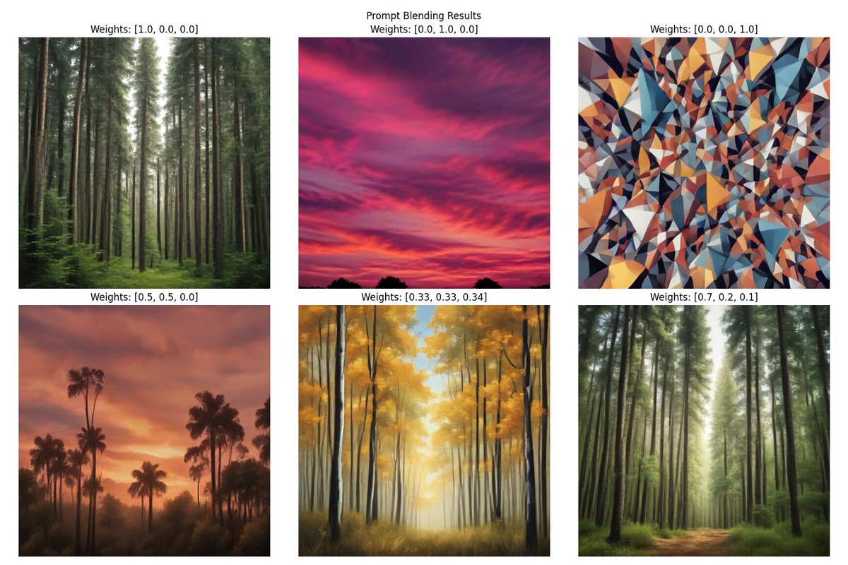
Linear interpolation: Notice how the forest trees incorrectly turn into palm trees in the middle frames.

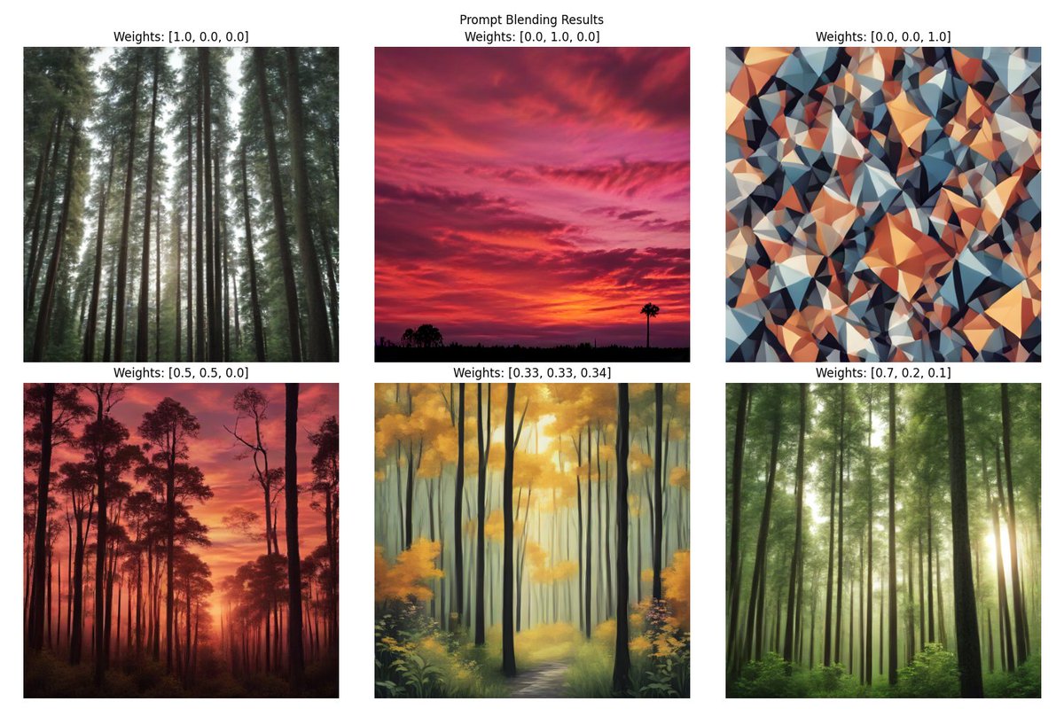
Spherical interpolation (slerp): The forest remains coherent throughout the transition.

The model can still decode visually-coherent images with linear interpolation, but the semantic content suffers because the embedded prompt representation passes through low-probability regions. Slerp maintains coherent semantics throughout the interpolation.

Further Resources

• Original GAN Paper, Goodfellow et al.
• NIPS 2016 GAN Tutorial by Goodfellow
• GAN Lab — Interactive 2D GAN visualization
• Google’s GAN Course
• The GAN Zoo — Catalog of GAN variants

This post is part of the Visual Recognition module at the Master in Computer Vision, taught at UAB and the Computer Vision Center (CVC).